Documents

Quarto - authoring and publishing tools for collaborative scientific writing

Lars Schöbitz

April 3, 2024

Anatomy of a Quarto document

Components

Metadata: YAML
Text: Markdown
Code: Executed via knitr or jupyter

Weave it all together, and you have beautiful, powerful, and useful outputs!

Literate programming

Literate programming is writing out the program logic in a human language with included (separated by a primitive markup) code snippets and macros.

---
title: "ggplot2 demo"
date: "5/23/2023"
format: html
---

## MPG

There is a relationship between city and highway mileage.

```{r}
#| label: fig-mpg

library(ggplot2)

ggplot(mpg, aes(x = cty, y = hwy)) + 
  geom_point() + 
  geom_smooth(method = "loess")
```

Metadata

YAML

“Yet Another Markup Language” or “YAML Ain’t Markup Language” is used to provide document level metadata.

---
key: value
---

Output options

---
format: something
---

---
format: html
---

---
format: pdf
---

---
format: revealjs
---

Output option arguments

Indentation matters!

---
format: 
  html:
    toc: true
    code-fold: true
---

YAML validation

Invalid: No space after :

---
format:html
---

Invalid: Read as missing

---
format:
html
---

YAML validation

There are multiple ways of formatting valid YAML:

Valid: There’s a space after :

format: html

Valid: format: html with selections made with proper indentation

format: 
  html:
    toc: true

Quarto linting

Lint, or a linter, is a static code analysis tool used to flag programming errors, bugs, stylistic errors and suspicious constructs.

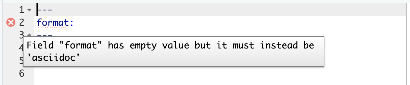
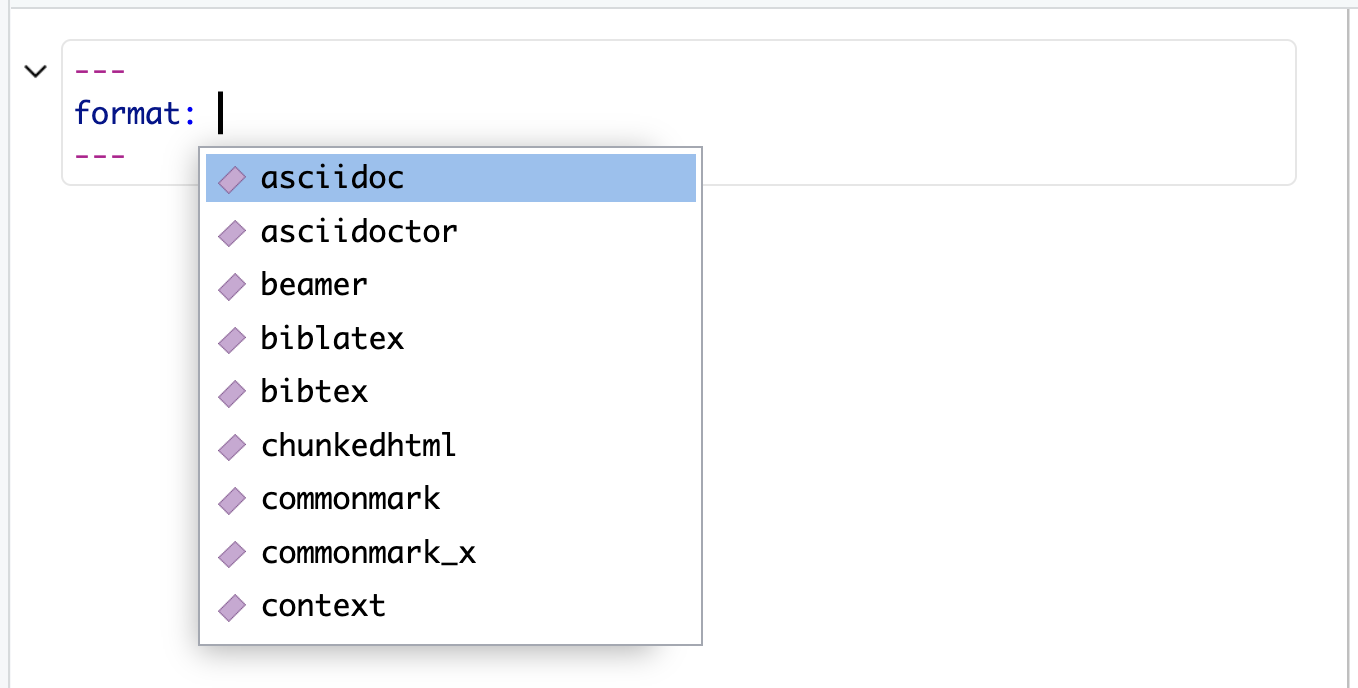
Linter showing message for badly formatted YAML.

Quarto YAML Intelligence

RStudio + VSCode provide rich tab-completion - start a word and tab to complete, or Ctrl + space to see all available options.

List of valid YAML fields

Many YAML fields are common across various outputs
But also each output type has its own set of valid YAML fields and options
Definitive list: quarto.org/docs/reference/formats/html

Text

Text Formatting

Markdown Syntax	Output
`italics and bold`	italics and bold
`superscript^2^ / subscript~2~`	superscript² / subscript₂
`~~strikethrough~~`	~~strikethrough~~
`verbatim code`	`verbatim code`

Headings

Markdown Syntax	Output
`# Header 1`	Header 1
`## Header 2`	Header 2
`### Header 3`	Header 3
`#### Header 4`	Header 4
`##### Header 5`	Header 5
`###### Header 6`	Header 6

Links

There are several types of “links” or hyperlinks.

Markdown

You can embed [named hyperlinks](https://quarto.org/),
direct urls like <https://quarto.org/>, and links to 
[other places](#quarto-anatomy) in 
the document. The syntax is similar for embedding an
inline image: 
![Penguins playing with ball](images/penguins-quarto-ball.png).

Output

You can embed named hyperlinks, direct urls like https://quarto.org/, and links to other places in the document. The syntax is similar for embedding an inline image: Penguins playing with ball .

Lists

Unordered list:

Markdown:

-   unordered list         
    -   sub-item 1         
    -   sub-item 1         
        -   sub-sub-item 1

Output

unordered list
- sub-item 1
- sub-item 1
  - sub-sub-item 1

Ordered list:

Markdown:

1. ordered list            
2. item 2                  
    i. sub-item 1          
         A.  sub-sub-item 1

Output

ordered list
item 2
1. sub-item 1
  1. sub-sub-item 1

Quotes

Markdown:

> Let us change our traditional attitude to the construction of programs: Instead of imagining that our main task is to instruct a computer what to do, let us concentrate rather on explaining to human beings what we want a computer to do. 
> - Donald Knuth, Literate Programming

Output:

Let us change our traditional attitude to the construction of programs: Instead of imagining that our main task is to instruct a computer what to do, let us concentrate rather on explaining to human beings what we want a computer to do. - Donald Knuth, Literate Programming

Your turn

Open markdown-syntax.qmd in RStudio.
Use the source editor mode
Follow the instructions in the document, then exchange one new thing you’ve learned with your neighbor.

07:00

Callouts

::: callout-note
Note that there are five types of callouts, including: 
`note`, `tip`, `warning`, `caution`, and `important`.
:::

Note

Note that there are five types of callouts, including: note, tip, warning, caution, and important.

More callouts

Warning

Callouts provide a simple way to attract attention, for example, to this warning.

Important

Danger, callouts will really improve your writing.

Caution

Here is something under construction.

Caption

Tip with caption.

Your turn

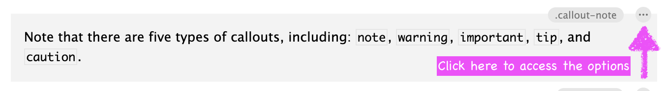
Open callout-boxes.qmd and render the document.
Using the visual editor mode, change the type of the first callouts box and then re-render.
Add a caption to the second callout box.
Make the third callout box collapsible. Then, switch over to the source editor mode to inspect the markdown code.
Change the format to PDF and re-render.

How to edit the options?

07:00

Footnotes

Numbering and formatting footnotes is supported.

Inline footnotes

Here is an inline note.^[Inlines notes are easier to write,
since you don't have to pick an identifier and move down to
type the note.]

Here is an inline note.¹

Use the source editor mode

The source editor mode is the recommended way to add footnotes.

Code

Anatomy of a code chunk

```{r}
#| label: penguins
#| message: false

library(tidyverse)
library(palmerpenguins)
library(knitr)

penguins |> 
  count(species) |> 
  kable()
```

species	n
Adelie	152
Chinstrap	68
Gentoo	124

Has 3x backticks on each end
Engine (r) is indicated between curly braces {r}
Options stated with the #| (hashpipe)

Code, who is it for?

The way you display code is very different for different contexts.
In a teaching scenario like today, I really want to display code.
In a business, you may want to have a data-science facing output which displays the source code AND a stakeholder-facing output which hides the code.

Showing and hiding code with `echo`

The echo option shows the code when set to true and hides it when set to false.

Tables and figures

In reproducible reports and manuscripts, the most commonly included code outputs are tables and figures.
So they get their own special sections in our deep dive!

Tables

Markdown tables

Markdown:

| Right | Left | Default | Center |
|------:|:-----|---------|:------:|
|   12  |  12  |    12   |    12  |
|  123  |  123 |   123   |   123  |
|    1  |    1 |     1   |     1  |

Use the source editor mode

The source editor mode is the recommended way to add markdown tables. These are tables, which are not generated from code.

Output:

Right	Left	Default	Center
12	12	12	12
123	123	123	123
1	1	1	1

Tables from code

The knitr package can turn data frames into tables with knitr::kable():

library(knitr)

penguins |> 
  count(species, island) |> 
  kable()

species	island	n
Adelie	Biscoe	44
Adelie	Dream	56
Adelie	Torgersen	52
Chinstrap	Dream	68
Gentoo	Biscoe	124

Tables from code

If you want fancier tables, try the gt package and all that it offers!

library(gt)

head(penguins) |> 
  gt() |>
  tab_style(
    style = list(
      cell_fill(color = "pink"),
      cell_text(style = "italic")
      ),
    locations = cells_body(
      columns = bill_length_mm,
      rows = bill_length_mm > 40
    )
  )

species	island	bill_length_mm	bill_depth_mm	flipper_length_mm	body_mass_g	sex	year
Adelie	Torgersen	39.1	18.7	181	3750	male	2007
Adelie	Torgersen	39.5	17.4	186	3800	female	2007
Adelie	Torgersen	40.3	18.0	195	3250	female	2007
Adelie	Torgersen	NA	NA	NA	NA	NA	2007
Adelie	Torgersen	36.7	19.3	193	3450	female	2007
Adelie	Torgersen	39.3	20.6	190	3650	male	2007

Figures

Markdown figures

![Penguins playing with a Quarto ball](images/penguins-quarto-ball.png)

Penguins playing with a Quarto ball

Subfigures

Markdown:

::: {#fig-penguins layout-ncol=2}

![Blue penguin](images/blue-penguin.png){#fig-blue width="250px"}

![Orange penguin](images/orange-penguin.png){#fig-orange width="250px"}

Two penguins

:::

Subfigures

Output:

Finding the figures to include

In places like markdown, YAML, or the command line/shell/terminal, you’ll need to use absolute or relative file paths:

Absolute = BAD: "/Users/lars/exercises" - Whose computer will this work on?

Relative = BETTER:
- "../ = up one directory, ../../ = up two directories, etc.
- /.. or / = start from root directory of your current computer

Figures with code

```{r}
#| fig-width: 4
#| fig-align: right

knitr::include_graphics("images/penguins-quarto-ball.png")
```

Referencing paths in R code

Use the here package to reference the project root, as here::here() always starts at the top-level directory of a .Rproj:

here::here()

[1] "/Users/lschoebitz/Documents/gitrepos/gh-org-quarto-ambition/website"

Figures from code

```{r}
ggplot(penguins, aes(x = species, fill = species)) +
  geom_bar(show.legend = FALSE)
```

Cross references

Help readers to navigate your document with numbered references and hyperlinks to entities like figures and tables.
Cross referencing steps:
- Add a caption to your figure or table.
- Give an ID to your figure or table, starting with fig- or tbl-.
- Refer to it with @fig-... or @tbl-....

Figure cross references

The presence of the caption (Blue penguin) and label (#fig-blue-penguin) make this figure referenceable:

Markdown:

See @fig-blue-penguin for a cute blue penguin.
![Blue penguin](images/blue-penguin.png){#fig-blue-penguin}

Output:

See Figure 2 for a cute blue penguin.

Table cross references

The presence of the caption (A few penguins) and label (#tbl-penguins) make this table referenceable:

Markdown:

See @tbl-penguins for data on a few penguins.
```{r}
#| label: tbl-penguins
#| tbl-cap: A few penguins

head(penguins) |> 
  gt()
```

Output:

See Table 1 for data on a few penguins.

head(penguins) |> 
  gt()

Table 1: A few penguins

species	island	bill_length_mm	bill_depth_mm	flipper_length_mm	body_mass_g	sex	year
Adelie	Torgersen	39.1	18.7	181	3750	male	2007
Adelie	Torgersen	39.5	17.4	186	3800	female	2007
Adelie	Torgersen	40.3	18.0	195	3250	female	2007
Adelie	Torgersen	NA	NA	NA	NA	NA	2007
Adelie	Torgersen	36.7	19.3	193	3450	female	2007
Adelie	Torgersen	39.3	20.6	190	3650	male	2007

Homework assignments

Homework

quarto-ambition.github.io/website/0-3-homework/index.html

Thanks! 🌻

Slides created via revealjs and Quarto: https://quarto.org/docs/presentations/revealjs/

Access slides as PDF on GitHub

All material is licensed under Creative Commons Attribution Share Alike 4.0 International.

Knuth, D. E. 1984. “Literate Programming.” The Computer Journal 27 (2): 97–111. https://doi.org/10.1093/comjnl/27.2.97.

Documents

Anatomy of a Quarto document

Components

Literate programming

Metadata

YAML

Output options

Output option arguments

YAML validation

YAML validation

Quarto linting

Quarto YAML Intelligence

List of valid YAML fields

Text

Text Formatting

Headings

Header 1

Header 2

Header 3

Header 4

Header 5

Header 6

Links

Lists

Quotes

Your turn

Callouts

More callouts

Your turn

Footnotes

Inline footnotes

Code

Anatomy of a code chunk

Code, who is it for?

Showing and hiding code with echo

Tables and figures

Tables

Markdown tables

Tables from code

Tables from code

Figures

Markdown figures

Subfigures

Subfigures

Finding the figures to include

Figures with code

Referencing paths in R code

Figures from code

Cross references

Cross references

Figure cross references

Table cross references

Homework assignments

Homework

Thanks! 🌻

Showing and hiding code with `echo`